Introduction
Greenhouse gas emissions are gas emissions caused by human activities; for example, carbon dioxide emits from burning fossil fuels for electricity and transportation (Sources of Greenhouse Gas Emissions, n.d.). Such emissions strengthen the greenhouse effect, which then results in climate change. Since the start of the industrial revolution from the mid-18th century to about 1830, the increase of industrial activities gradually led to the warming up of the climate system on Earth, and to this day, climate change has become a growing concern (Industrial Revolution, 2022; Tiseo, 2021).
In this project, we aim to look at some variables related to greenhouse gas emissions and observe if there is any relationship between them. Specifically, we want to investigate the significance of the relationship between a country’s GDP per capita and its CO2 emissions, and the significance of the relationship between time and CO2 emissions for a multitude of countries.
To achieve this, we found the Emissions data set, a CSV file from the CORGIS Dataset Project, about greenhouse gas emissions by country (Kafura, 2019). The data file from the CORGIS Dataset Project is originally obtained from the Emissions Database for Global Atmospheric Research database. It includes 8385 observations and 12 variables: country, year (1970-2012), and variables related to gas emissions, which are
- emissions of: CO2 (carbon dioxide), N2O (nitrous oxide), and CH4 (methane);
- emissions from: the power industry, the infrastructure of buildings, means of transportation, other industrial combustion, and other sectors;
- the ratio of: greenhouse gas emissions per $1,000 of GDP, and emissions each person.
All variables above are numeric, either measuring emission or ratio. Emissions of CO2 are measured in kilotons, and all others are measured in equivalent kilotons of CO2.
Methods and Results
Time, GDP, and CO2 Emissions
The first observation is between time and CO2 emissions. Time will be measured in the years from 1970 to 2012, and CO2 emissions will be expressed as the greenhouse gasses emitted through human activities measured in kilotons. The country of the Maldives will be used as a control variable for the first two data explorations. The Maldives was chosen out of interest because in the time period of 2001-2020, the Maldives experienced a vast amount of deforestation and a significant loss of tree cover (Statistics about Forests in Maldives, n.d.). We became intrigued to investigate the CO2 emissions of kilotons in the Maldives over time.
hide
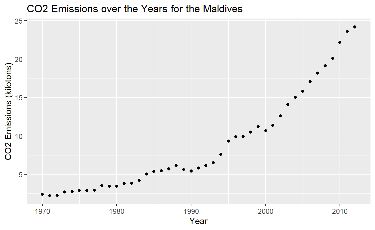
When initially looking at the graph, we noticed that as time increased, so did the CO2 emissions; the CO2 emissions were increasing exponentially. There was a significant increase in CO2 emissions in the later years. This aroused our interest to find out if there was a significant reason why this had occurred, such as, if there was an increase in some factor that related to CO2 emissions. An increase in factory farming increases the emission of several greenhouse gasses, and factory farming is related to economic development, so we decided to create a scatter plot to visualize the relationship between the ratio of emissions to GDP and CO2 emissions.
hide
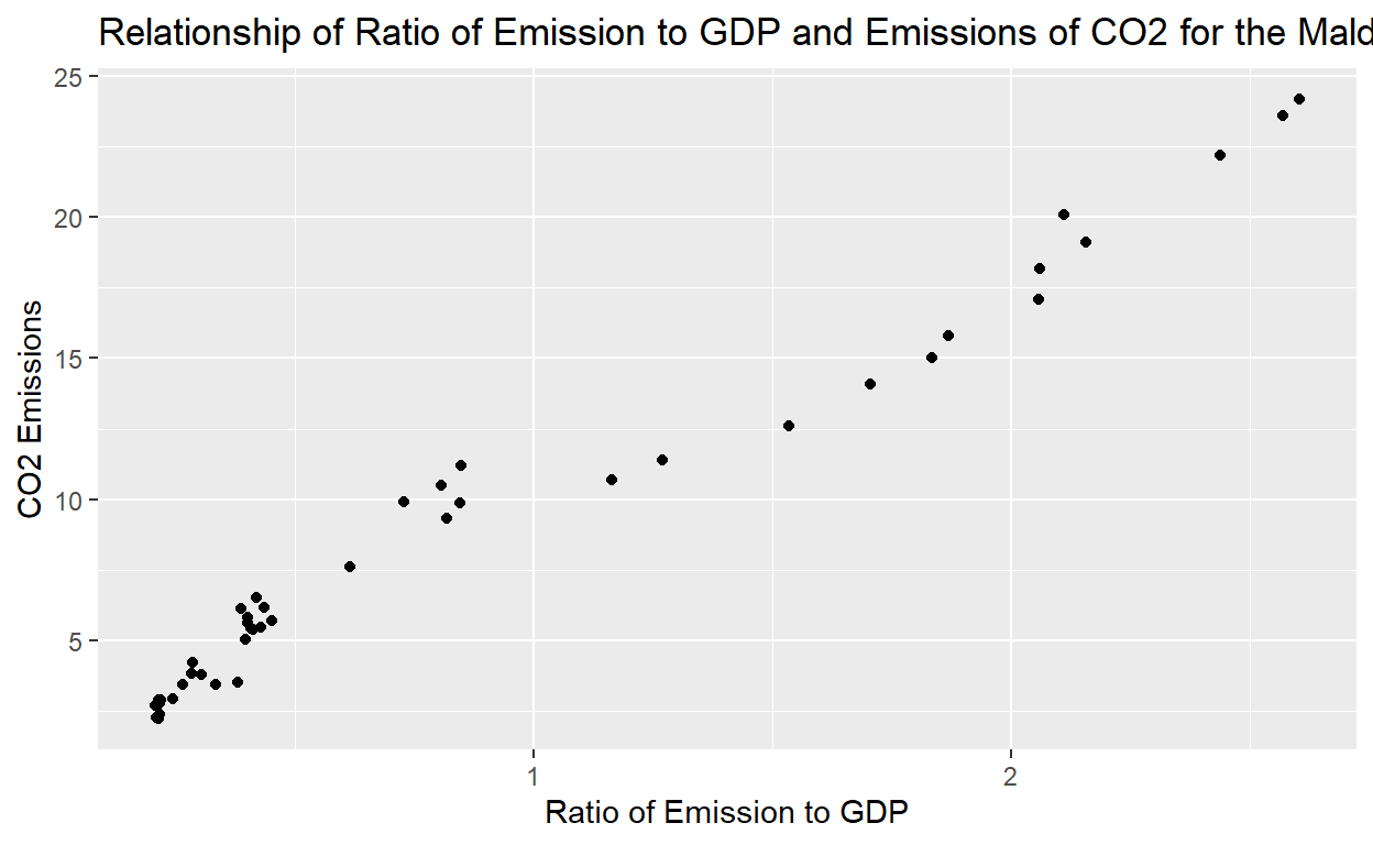
There is a positive association between the ratio of emissions to GDP and CO2 Emissions for the Maldives, and there were no significant outliers presented in the graph. In the next section, we will investigate if there was a significant relationship between these two variables.
Hypothesis Test about GDP and CO2 Emissions
First, we found the correlation between the ratio of emissions to GDP and CO2 emissions for the country of the Maldives.
# A tibble: 1 × 1
  r_free
   <dbl>
1  0.985
Evidently, the correlation is very close to 1 which indicates a strong positive association between the two variables. Then we conducted a linear model hypothesis test to test and see if a linear model is appropriate for these variables. We stated the equation as \(y_{\text{CO}2} = \beta_0 + \beta_1x_{\text{GDP}}\), with \(y_{\text{CO}2}\) as the CO2 emissions response variable, \(\beta_0\) as the intercept, and \(\beta_1\) as the slope predicted by the null and alternate hypothesis.
\(H_0\): There is no linear relationship between the ratio of emissions to GDP and CO2 emissions for the country of the Maldives. The expected slope of the linear model is \(\beta_1 = 0\).
\(H_1\): There is a linear relationship between the ratio of emissions to GDP and CO2 emissions for the country of the Maldives. The expected slope of the linear model is \(\beta_1 \neq 0\).
hide
Call:
lm(formula = CO2 ~ ratio_per_GDP, data = .)

Residuals:
    Min      1Q  Median      3Q     Max
-1.7224 -0.7504 -0.2121  0.8579  2.5467

Coefficients:
              Estimate Std. Error t value Pr(>|t|)
(Intercept)     1.6989     0.2593   6.552 7.09e-08 ***
ratio_per_GDP   8.1951     0.2226  36.813  < 2e-16 ***
---
Signif. codes:  0 '***' 0.001 '**' 0.01 '*' 0.05 '.' 0.1 ' ' 1

Residual standard error: 1.117 on 41 degrees of freedom
Multiple R-squared:  0.9706,    Adjusted R-squared:  0.9699
F-statistic:  1355 on 1 and 41 DF,  p-value: < 2.2e-16
The multiple R-squared value was also very close to 1 which signifies that the proportion of variability that the linear model is 0.976. Additionally, the p-value was also very close to 0 which indicates that there is strong evidence against the null hypothesis, thus indicating that a linear model is an appropriate fit for the variables of GDP and CO2 emissions for the country of the Maldives. Based on the results presented, as the GDP increases by one unit, the CO2 emissions in the Maldives increases by 8.1951 units.
Time and CO2 Emissions for Multiple Countries
We examined which countries have the highest average CO2 emissions and how the CO2 emission changed over the years. This value was calculated by taking an average of the CO2 emissions of each country over the years.
hide
emissions %>% group_by(country) %>%
  summarize(avg_CO2 = mean(CO2)) %>%
  arrange(desc(avg_CO2)) %>%
  head(25) %>%
  ggplot(aes(x = avg_CO2, y = reorder(country, avg_CO2))) +
    geom_bar(stat = "identity") +
    labs(title = "Top Countries by Highest Average CO2 Emissions",
         x = "Average CO2 Emission", y = "Country")
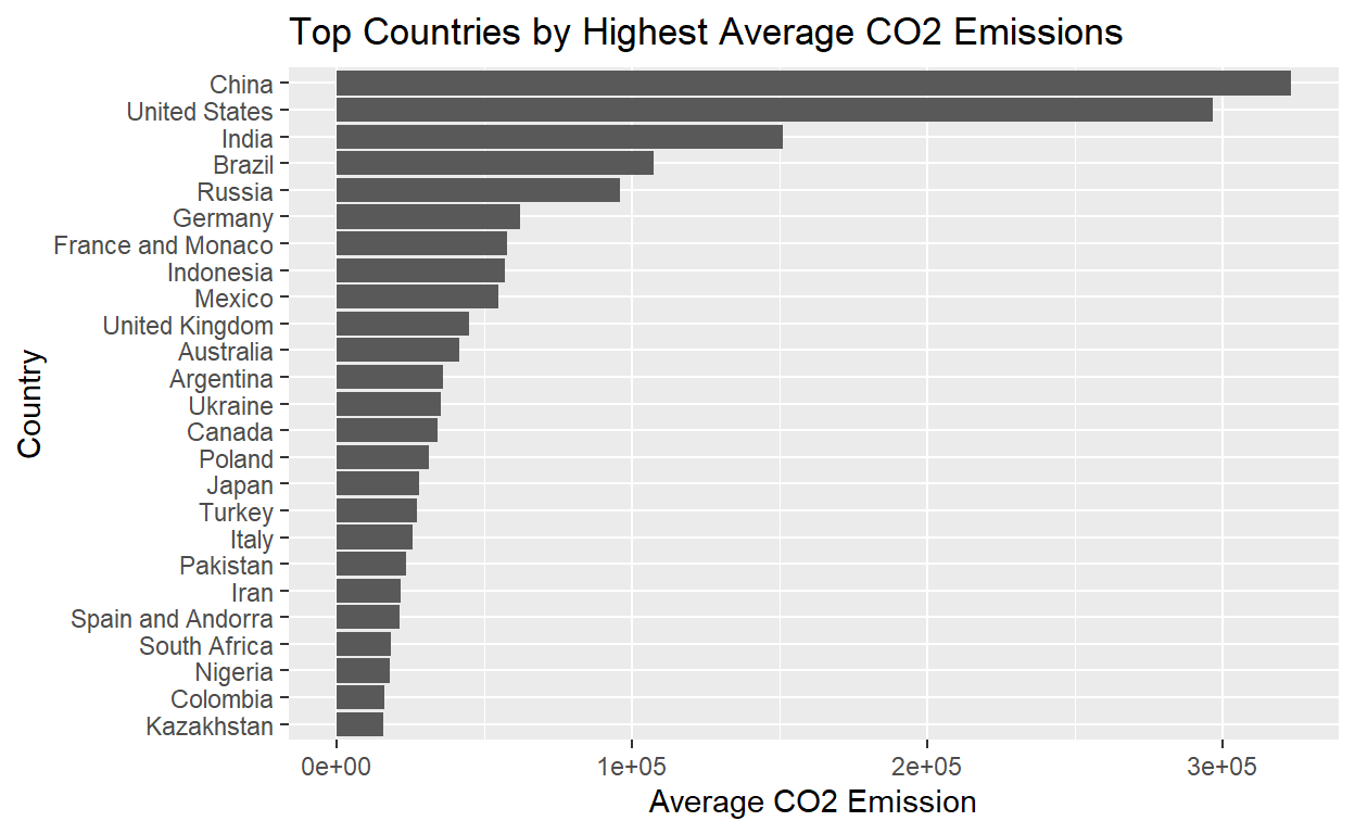
As the bar plot shows, China, United States, India, Brazil, and Russia are the top 5 countries with the highest CO2 emissions through the years. China and United States have especially high emission. Then the next plot compares the change of emissions overtime of these top 5 countries.
hide
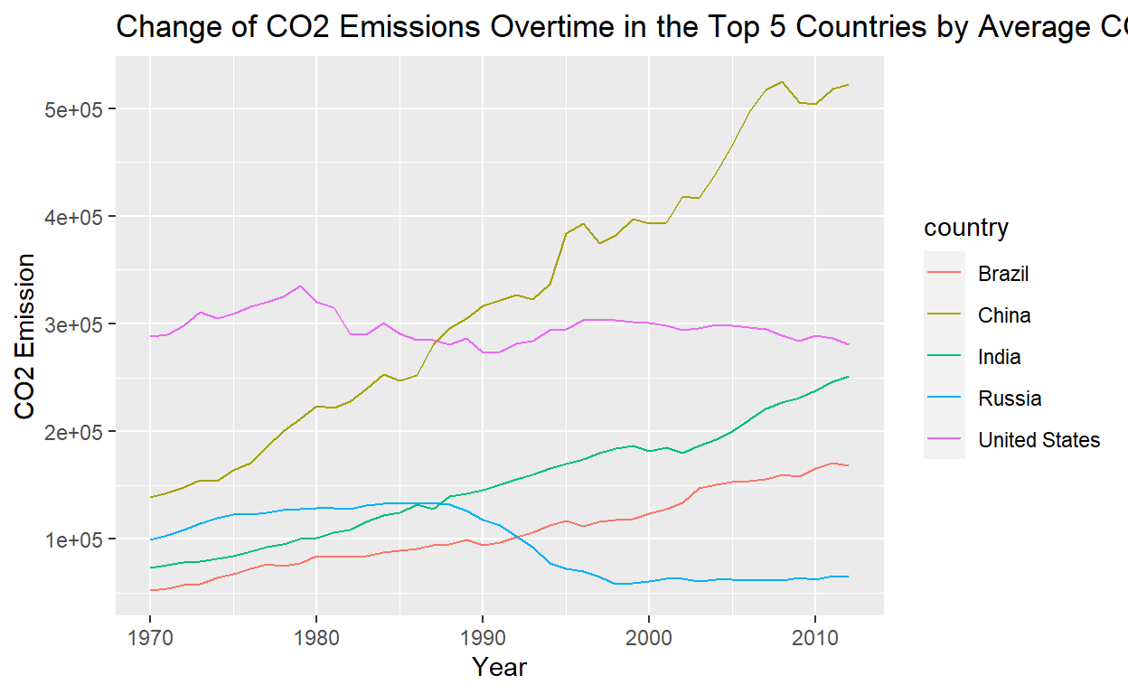
In the time period after 1985 and around 1990, we see multiple crossovers: between United States and China, Russia and India, and Russia and Brazil. The trends in China, India, and Brazil are increasing, while the trends in United States and Russia are slightly decreasing. This could be due to the increase in the amount of factories and industries in the developing countries and a relatively stable trend in the developed countries.
To fit a model to predict CO2, we used multiple linear regression covariating the variables of emissions from all the industries. That is, we want to predict the significance of the coefficients of the formula \(y_{\text{CO}2} = \beta_0 + \sum{\beta_ix_i}\), where \(x_i\) are variables of emissions from power industries, buildings, transportation, other industries, and other sectors. Since these variables are all measured in equivalent kilotons of CO2, it is expected that all variables will be significant. Indeed, the low p-values show that they are all significant predictors.
Call:
lm(formula = CO2 ~ power_ind + buildings + transport + other_ind +
    other_sect, data = emissions)

Residuals:
    Min      1Q  Median      3Q     Max
-176806   -2115   -1750    -107  148119

Coefficients:
            Estimate Std. Error t value Pr(>|t|)
(Intercept) 2108.903    155.396   13.57   <2e-16 ***
power_ind    -45.331      3.772  -12.02   <2e-16 ***
buildings    198.794      6.436   30.89   <2e-16 ***
transport     68.067      4.883   13.94   <2e-16 ***
other_ind     94.355      5.467   17.26   <2e-16 ***
other_sect   254.433     14.187   17.93   <2e-16 ***
---
Signif. codes:  0 '***' 0.001 '**' 0.01 '*' 0.05 '.' 0.1 ' ' 1

Residual standard error: 13570 on 8379 degrees of freedom
Multiple R-squared:  0.8651,    Adjusted R-squared:  0.865
F-statistic: 1.074e+04 on 5 and 8379 DF,  p-value: < 2.2e-16
We then conducted the same method using the same variable but predicting the N2O emissions.
Call:
lm(formula = N2O ~ power_ind + buildings + transport + other_ind +
    other_sect, data = emissions)

Residuals:
    Min      1Q  Median      3Q     Max
-600241   -8153   -7173   -2395  613738

Coefficients:
            Estimate Std. Error t value Pr(>|t|)
(Intercept) 8160.426    647.054  12.612  < 2e-16 ***
power_ind   -213.827     15.707 -13.614  < 2e-16 ***
buildings    937.241     26.798  34.974  < 2e-16 ***
transport     -2.084     20.334  -0.102  0.91837
other_ind     65.746     22.764   2.888  0.00389 **
other_sect  1433.964     59.075  24.274  < 2e-16 ***
---
Signif. codes:  0 '***' 0.001 '**' 0.01 '*' 0.05 '.' 0.1 ' ' 1

Residual standard error: 56500 on 8379 degrees of freedom
Multiple R-squared:  0.7657,    Adjusted R-squared:  0.7656
F-statistic:  5477 on 5 and 8379 DF,  p-value: < 2.2e-16
In this model, the p-values for emissions from transportation and other industries are larger than others and larger than the previous model for CO2, with the one for transportation especially high. So the emissions from means of transportation is not a statistically significant predictor for N2O emissions.
Conclusions
The main objectives of this project were to investigate the significance of the relationship between GDP per Capita and CO2 emissions for the country of the Maldives as well as to investigate the significance of the relationship between time and CO2 emissions for a variety of countries. Our findings suggested that there is a significant linear relationship between the GDP per Capita and CO2 emissions for the Maldives, and that emissions from transportation are not a significant predictor for N2O emissions. If we had more time and resources for further research, we could have investigated other types of emissions in the Maldives such as methane and nitrous oxide for more insightful conclusions. Additionally, this project solely focused as GDP per Capita as an explanatory variable. With more time, this project could have focused more on other explanatory variables that were present in the data set such as power industries, infrastructure, and transportation.
Class Peer Reviews
Reviewer 1
- State the authors’ objectives and the general questions that the authors are considering. Do the results and figures support the conclusions made in the report?
The authors are interested in looking at the significance of the relationship between a country’s GDP per capita and its CO2 emissions, as well as the significance between time and CO2 emissions. The results and figures, such as the bar graphs and linear regressions, do support the conclusions made in the report, which are that there is a linear relationship between the GDP per capita and C02 emissions for the Maldives, and that emissions from transportation is not a significant predictor for N2O emissions.
- Discuss the foundations of data visualizations relative to the figures presented in the report.
The data visualizations the authors use are primarily bar graphs, to visualize the countries with the highest average CO2 emissions, and line graphs, to visualize the change in CO2 emissions overtime. They additionally use a scatter plot to show the ratio of emissions to GDP in the Maldives. They also include a scatterplot for the CO2 emissions over the years for the Maldives.
- State 3 things that are strong about their report and 2 things that can be improved.
The use of null and alternative hypotheses, the CO2 emissions graph that shows CO2 emissions overtime, and the writing of the report all work to make the report very clear. I would be curious to see data from other countries besides the Maldives. I’m also a little confused to how the two sections of the report tie together (maldives and transportation emissions)
Reviewer 2
- State the authors’ objectives and the general questions that the authors are considering. Do the results and figures support the conclusions made in the report?
The main objective of this project is to study the association between greenhouse gas emissions and other variables which might be relevant. The greenhouse gas studied in the project is CO2 and the explanatory variable chosen is the GDP per capita. With the time series graph of the raw data, it is expected that these two variables would have a positive relationship. The conclusion agrees with it. The linear model we have have a positive coefficient of 8.1951 with a astronomically small p-value.
- Discuss the foundations of data visualizations relative to the figures presented in the report.
The first graph is a time series plot of the CO2 emissions in Maldives from 1970 to 2020. It is nice and easy to understand. The second graph is a scatter plot between the ratio of emissions to GDP and CO2 emissions. There is a crowd of data points at the bottom left corner of the graph. Maybe it is better to change the transparency of the points for a better visualization. Also, the last few words of the title of this plot is hidden in the background. The third plot is a bar plot of the average CO2 emissions for the top 25 countries. One thing I would add to this graph is the number of countries shown in the graph. The fourth plot is a line graph of the change of CO2 emissions overtime of the top 5 countries. The size of the y-axis is a little confusing. It is a change of CO2 emission, so I would not expect it to be on a magnitude of 105. It is better to have a couple of sentence explaining why this is true.
- State 3 things that are strong about their report and 2 things that can be improved.
Three things that are strong. First, the visualizations are easy to understand in general. Second, the linear models we get have small p-values for the coefficients. Third, the tone of this project is objective.
Two things to improve. First, we can add visualizations for other greenhouse gases. They can be put at the beginning of the method section, or with the linear model we have for the N2O. Second, there is no explanation for the coefficient generated by the last two linear models. It would be great to have some words about them.